Comparison of 2009 Volkswagen Polo 1.2 R6 and 2012 Toyota Yaris Hybrid fuel consumption under economic driving conditions

Sven Mahler

Fuelcons | Real world fuel consumption data and analysis | www.fuelcons.com | Mahler@fuelcons.com

ABSTRACT

The aim of the present study was to compare the average fuel consumption (per tank of fuel) of the gasoline-powered 2009 Volkswagen Polo 1.2 R6 (Polo) with that of the 2012 Toyota Yaris Hybrid (YHSD) under consideration of underlying average temperatures and speeds. Both vehicles were sequentially driven by the same driver on comparable routes and with the intention to save fuel. The latter included the application of hypermiling techniques, especially when driving the Polo. Covered distances were 62,629 km (Polo) and 50,069 km (YHSD). Overall, the average fuel consumption of the YHSD was 19% lower than that of the Polo (4.10 vs. 5.04 L/100 km). Using multiple linear regression analysis, the effect of average temperature on average fuel consumption was found to be comparable for both vehicles (− 0.0408 L/100 km and − 0.0397 L/100 km per increase of one degree Celsius for the Polo and the YHSD, respectively). In contrast, an opposing impact of average speed was observed (− 0.0185 L/100 km [Polo] and + 0.0249 L/100 km [YHSD] for each additional km/h in average speed). The results are discussed in light of type-approval- and real world fuel consumption figures.     

Please cite this article as:
Mahler S. (2020). Comparison of 2009 Volkswagen Polo 1.2 R6 and 2012 Toyota Yaris Hybrid fuel consumption under economic driving conditions. Fuelcons-2020-1. Available at: www.fuelcons.com/1e1-6-polo-vs-yhsd/

Copyright:
This article is available under the Creative Commons CC-BY-SA license and permits distribution, adaption and reproduction in any medium, even commercially, provided the original work is properly cited. If you remix, transform, or build upon the material, you must distribute your contributions under the same license as the original.

INTRODUCTION

According to official New European Driving Cycle (NEDC) ratings, the (combined) fuel consumption (FC) of the 2012 Toyota Yaris Hybrid (YHSD) is 36% lower than that of the 2009 Volkswagen Polo 1.2 R6 (Polo) (3.5 vs. 5.5 L/100 km) [1,2]. Due to limitations of the NEDC, this driving cycle has recently been replaced by the more realistic Worldwide harmonized Light vehicles Test Procedure (WLTP) [3]. Compared to test stand-based driving cycles, however, real world FC databases may generally provide more reasonable data [4]. Based on information available in the Spritmonitor database, YHSD-related savings shrink to ~ 25% (4.8 vs. 6.4 L/100 km) [5,6]. Based on these data, the 2009 NEDC rating of the Polo (+ 0.8 L/100 km [+ 15%] under real world conditions) appears to be more realistic than that of the 2012 YHSD (+ 1.3 L/100 km [+ 37%]).

However, also available real-world data should be treated with caution. For example, it appears to be likely that, in comparison to the Polo, the YHSD is more often driven by economic drivers at lower speeds [7]. Furthermore, it may be true that especially drivers that take care of (lower) fuel consumption enter more (reliable) data into fuel consumption databases. Indeed, while there are currently 276 YHSD-accounts on Spritmonitor with a minimum mileage of 50,000 km, the number of that for the Polo is only 33 [5,6].

These exemplary factors illustrate that best possible comparison of the FC of different vehicles requires unbiased data, similar route characteristics and comparable driving styles. In the present study, the average FC per tank of fuel (average FC) of the YHSD and the Polo, both driven under economic driving conditions and on comparable routes, were determined in dependence of underlying average temperature and speed.

MATERIALS AND METHODS

Vehicles

2012 Toyota Yaris Hybrid / Life (YHSD) [1]:

Propulsion: petrol powered ‘full’ hybrid electric system, ‘Hybrid Synergy Drive [HSD]’; primary engine: Atkinson cycle ICE, 55 kW (75 PS), 4 cylinders, 1.5 l capacity. Secondary main engine (MG2): 45 kW (61 PS) electric motor / generator. Traction battery: nickel-metal hydride (NiMH) battery pack, 144 V, 6.5 Ah (0.9 kWh), power: 19 kW (26 PS). Combined power of the hybrid system: 55 kW (ICE) + 19 kW (battery) = 74 kW (101 PS). Transmission: Planetary gear unit (e-CVT).

Fuel tank capacity: 36 liters.

Tyres: Summer / Winter: both 175/65 R15.

Tyre pressure: between 2.8 bar (40.6 psi) and 3.0 bar (43.5 psi) throughout the year.

Official FC / emission figures (NEDC): FC: 3.1 / 3.5 / 3.5 l/100km (urban / extra-urban / combined). Carbon dioxide emissions: 79 g/km.

2009 Volkswagen Polo V / 6R 1.2 Comfortline (Polo) [2]:

Propulsion: petrol powered four-stroke internal combustion engine (ICE), 51 kW (69 PS), 3 cylinders, 1.2 l capacity. Transmission: five-speed manual gear box.

Fuel tank capacity: 45 liters.

Tyres: Summer: 185/60 R15 / winter: 165/80 R14.

Tyre pressure: between 2.8 bar (40.6 psi) and 3.0 bar (43.5 psi) throughout the year.

Official FC / emission figures (NEDC): FC: 7.3 / 4.5 / 5.5 l/100km (urban / extra-urban / combined). Carbon dioxide emissions: 128 g/km.

Routes and driving styles

Both vehicles were mainly driven on the following routes, albeit with different frequencies: a 7 km urban short-trip, a 75 km combined urban (10 km) / extra-urban (freeway; 65 km) intercity trip (highly prone to congestions) as well as a 150 km combined freeway / rural road trip. Economic driving conditions generally included: (I) anticipatory driving, (II) a maximum speed of 100 km/h (according to speedometers), (III) use of cruise control (extra-urban), (IV) truck slipstreaming on freeways, (V) turned off air-conditioning, and (VI), whenever possible, no use of the car heater during warmup of the ICE. No extra-urban pulse-and-glide was systematically performed. The ECO-mode of the YHSD was always activated. Polo-specific measures included: (I) manual stop of the engine at red traffic lights, and (II) engine-off coasting [8]. However, the engine was turned off only when the (ICE temperature-dependent) idle fuel consumption was 0.6 L/hour or lower.

Acquisition of data

During the data acquisition periods, some or all of the following data were recorded during each refueling stop: date of refueling (date), amount of fuel tanked / needed for complete fill-up (pump vol [L]), and, as given by the trip computer (TC), the distance covered (distance [km]) and the average speed (km/h) since the last complete fill-up. Average FC (L/100 km) was calculated as follows: pump vol*100/distance. In contrast to the Polo, the TC of the YHSD did not provide two independent memories to allow the recording of overall data in parallel to that of single trips. Furthermore, the average speed was automatically reset after each reboot of the vehicle. Thus, the average speed since the last complete fill-up was derived from recorded (single)-trip data whereat the calculated average speed was only considered acceptable when representing at least 95% of the total distance covered. The average temperature (°C) between refuelings was esteemed as the average temperature in Germany during this period. Corresponding data were obtained from WolframAlpha (www.wolframalpha.com) using the following inquiry: ‘Average temperature Germany between DD/MM/YYYY and DD/MM/YYYY’. A summary of available data as relevant for the present study is given in Table 1.

Table 1. Basic (meta)-information and available data

Meta-information	Polo	YHSD
Vehicle driven from – to (month/year)	09/2009 – 01/2013	01/2013 – to date
Data acquisition period (month/year)	11/2009 – 01/2013	02/2013 – 12/2015
Total distance covered	62,629 km	50,069 km
Total amount of fuel consumed	3,158 L	2,053 L
Refuelings (complete fill-ups)	75 (74)	61 (61)
Average amount of fuel tanked	42.67 L	33.66 L
Average distance driven / tank of fuel	835 km	820 km
Overall fuel consumption*	5.04 L/100 km	4.10 L/100 km
Number of available data sets	Polo	YHSD
FC & avg. temp	73	61
FC & avg. temp & avg. speed	32	36

*based on total amount of fuel consumed and total distance covered.

Handling of data, analysis, and graphical presentation

All basic data (date, distance, pump vol) were entered into the ‘Spritmonitor’ database [9,10]. Microsoft Excel® 2013 was used for data analysis and graphical presentation. For identification of outliers, the 1.5x interquartile range (IQR) rule (Tukey’s Boxplot method) was followed as described elsewhere [11]. Microsoft PowerPoint® 2013 was used for multi-panel figure assembly and generation of graphic-files [12]. Besides the manual calculations described below, Multiple Linear Regression Analysis was done as described below and by using free (R-based) online software that computes a multiple regression model based on the Ordinary Least Squares method [13].

RESULTS

All single data sets (average FC, -temperature, and -speed) were independently checked for outliers using the 1.5x IQR rule [11]. Accordingly, one outlying average speed information (82.9 km/h) for the YHSD was excluded from further analysis.

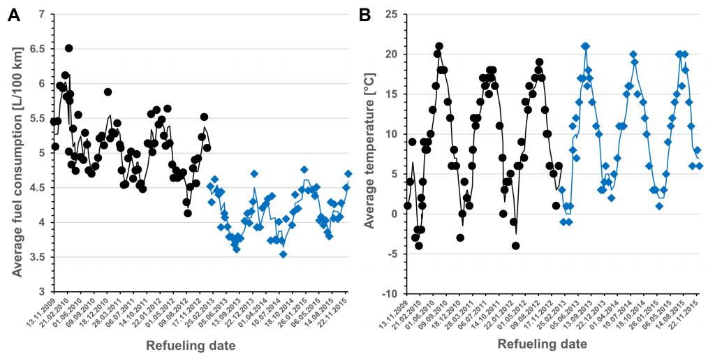
The progression of average FCs over the years are shown in Figure 1A. For both vehicles, a clear inverse dependence of fuel consumption on the average temperature (Fig. 1B) was observed.

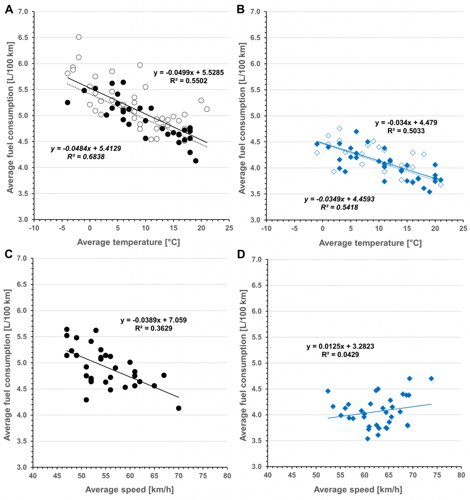
The correlations of corresponding data are shown in Figures 2A (Polo) and 2B (YHSD). Additional information on average speed was available for a subset of data (filled symbols in Figs. 2A/B). The correlations between average speed and average FC are shown in Figures 2C (Polo) and 2D (YHSD). While the average FC of the Polo dropped with increasing average speed, a reverse trend was observed for the YHSD.

The basic statistical characteristics of the available complete datasets (containing information on both, average temperature and -speed) are summarized in Table 2.

Table 2. Basic statistical information of available datasets.

	Polo				YHSD
Parameter	min	max	M	x	min	max	M	x	p
Avg. FCa	4.13	5.64	4.87	4.92	3.54	4.70	4.05	4.07	<0.001
Avg. temp.b	-4	19	10.0	10.3	-1	21	11.0	11.2	0.535
Avg. speedc	47	70	54.0	55.1	52.4	73.8	62.8	62.8	<0.001

^a L/100 km; ^b °C; ^c km/h, M: median, x: mean

For both vehicles, calculated median and mean values were found to be similar for all variables, assuming a normal distribution of underlying data. Thus, the Student’s t-Test was applied in order to test for relevant differences, with a p-value of < 0.05 deemed as statistically significant [14]. In brief, a p-value represents the probability of the observed result occurring if the so-called ‘null hypothesis’ were true [15]. In the present context, the ‘null hypothesis’ refers to the assumption that there is no difference between e.g. the average FC of the Polo and the YHSD. 

Accordingly, with a p-value of < 0.001, the lower mean average FC of the YHSD in comparison to that of the Polo was found to be clearly statistically significant. Regarding the underlying conditions, the average temperatures were found to be comparable (p=0.535) for both vehicles while the YHSD was driven at significantly higher average speeds (p<0.001).

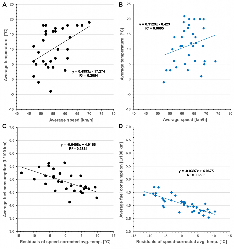
The linear trend lines shown in Figure 2 reflect the correlations between average temperature or average speed and average FC. However, correction of these data, that is the removal of the effects of average speed or average temperature, respectively, was needed to more accurately assess the respective isolated impact of these factors. Indeed, as shown in Figure 3A, the average speed gained with the Polo was positively correlated with average temperature. For the YHSD, a similar but less pronounced trend was observed (Fig. 3B).

In order to avoid overfitting of data, simple linear interpolation was chosen for both, data correction and final interpretation.

For the removal of the effects of average speed from average temperature data shown in Figures 2A (Polo) and 2B (YHSD), the respective formulas shown in Figures 3A and 3B were applied. These formulas delineate the interpolated linkage between average speed (x, horizontal axis) and average temperature (y, vertical axis). Thus, when subtracting these interpolated temperature values from the respective original average temperature values, the resulting residuals represent the speed-corrected average temperatures.

Plotting of average fuel consumptions over speed-corrected temperature residuals finally revealed the correlations shown in Figures 3C (Polo) and 3D (YHSD). According to the respective linear interpolation functions, for each additional degree (°C) of average temperature, the average FC of the Polo decreased by 0.0408 L/100 km while that of the YHSD decreased by 0.0397 L/100 km.

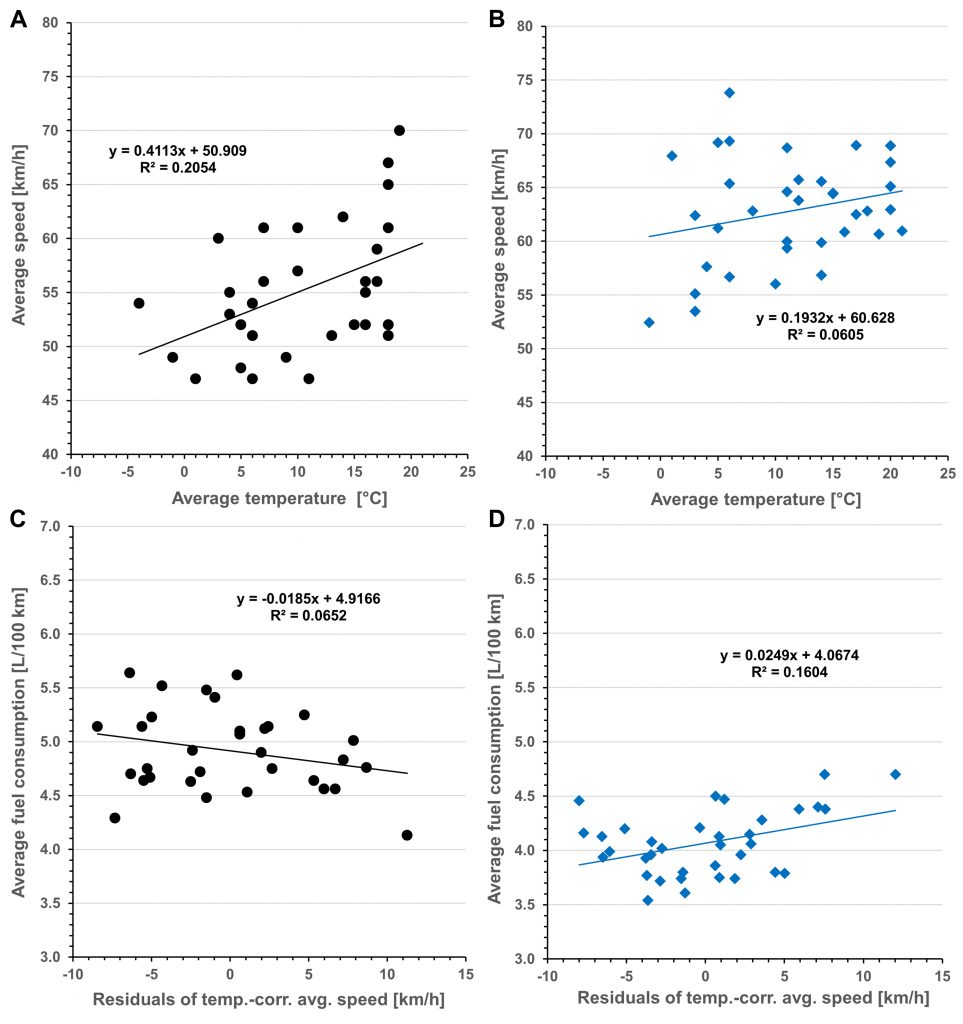
For analogous correction of average speed data for underlying average temperature, the formulas based on transposed data as shown in Figures 4A and 4B were applied. The correlations between temperature-corrected speed data (residuals) and average FC are shown in Figures 4C (Polo) and 4D (YHSD). Referring to the slopes of the linear interpolations, it could be concluded that the average FC of the Polo decreased by 0.0185 L/100 km while that of the YHSD increased by 0.0249 L/100 km for each additional km/ h of average speed.

Multiple linear regression analysis is a useful tool for the prediction of an unknown value (dependent variable) that depends on two or more known (potentially interacting) variables (independent variables).

In general, multiple linear regression analysis estimates (interpolates) a linear equation of the form:

y = a + b₁*x₁ + b₂*x₂ + …. + b_n*x_n [16].

Based on the conditions and findings of the present study, the corresponding formula reads

FC = 6.36 – 0.0408*temp – 0.0185*speed (equation #1)

for the Polo and

FC = 2.95 – 0.0397*temp + 0.0249*speed (equation #2)

for the YHSD,

whereat ‘FC’ represents the average FC, ‘temp’ the average temperature, and ‘speed’ the average speed. The constants ‘a’ could be easily calculated based on the respective mean values of ‘avg. FC’, ‘avg. temp’, and ‘avg. speed’ data shown in Table 2.

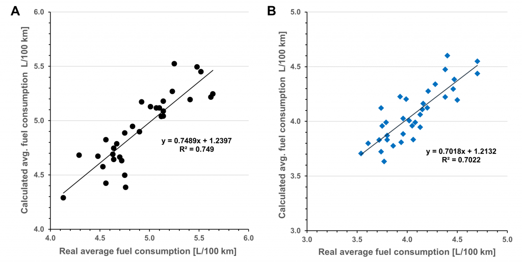
Using equations #1 and #2, interpolated average FC values were calculated and compared to the real values. As shown in Figures 5A and 5B, there was high correlation of data related to the Polo and the YHSD, respectively. The given R-squared values reflect the proportion of variation explained by the established linear interpolation models. Accordingly, one can conclude that the combination of average temperature and average speed explain ~75% and ~70% of the overall variation in average FC observed for the Polo and the YHSD, respectively.

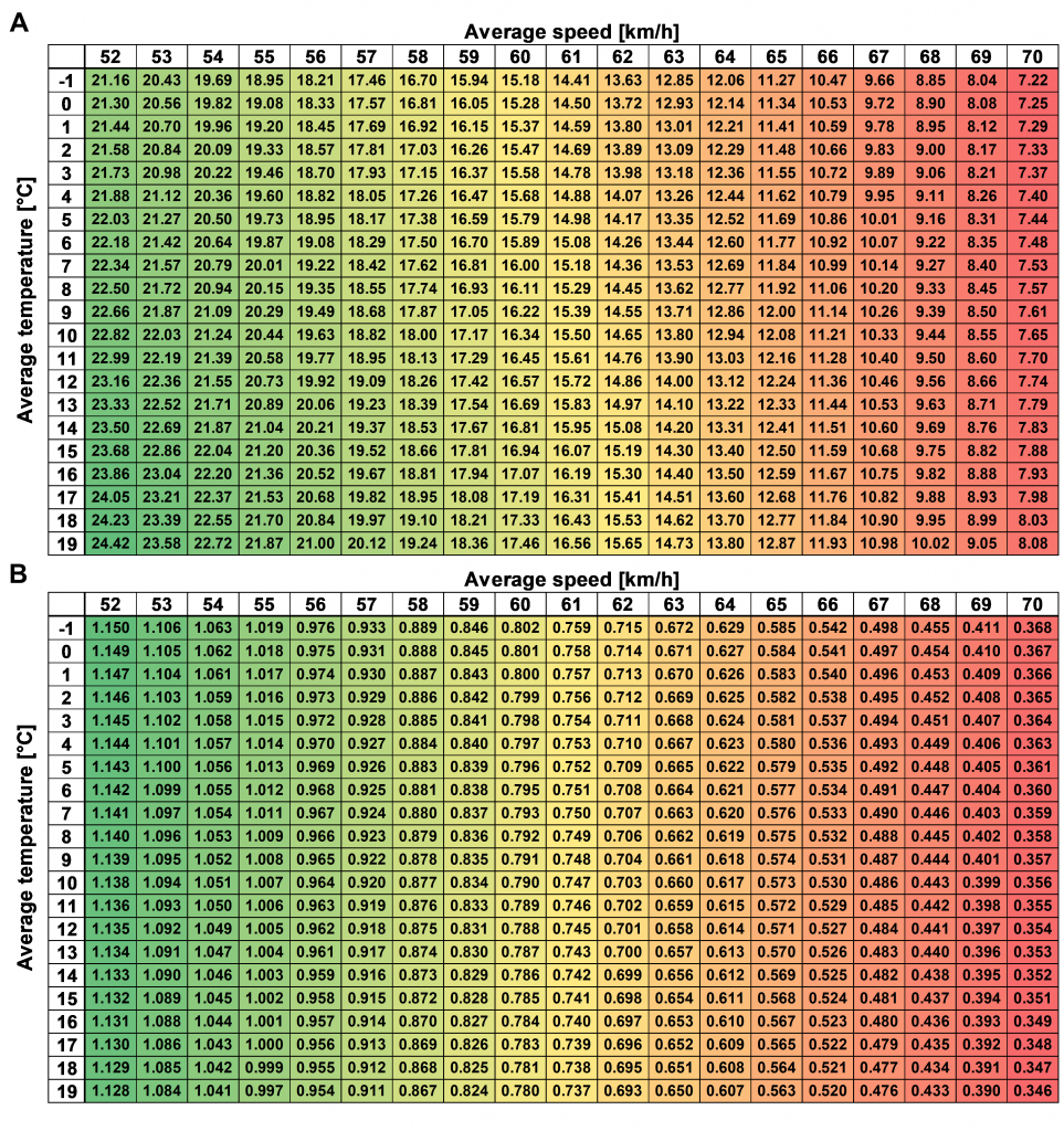
Despite the remaining uncertainties, equations #1 and #2 were applied to calculate the relative savings of YHSD average FC in comparison to that of the Polo in dependence of average temperature and speed. In order to avoid extrapolations, only the average temperature and -speed ranges covered by both vehicles were considered. As shown in Figure 6A, the relative savings ranged from 24.4% at lowest average speed and highest -temperature down to 7.2% under opposite conditions. The corresponding absolute savings are shown in Figure 6B.

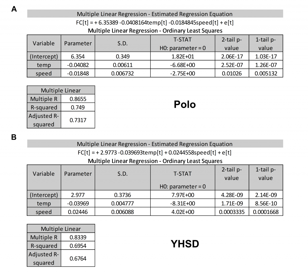
In order to confirm the data analysis described above, multiple regression analysis was also done using a corresponding online tool based on the Ordinary Least Squares method [13]. The obtained results are shown in Figure 7. Besides the established similar linear equations, the online tool also returned statistical key information, including (2-tail) p-values. As already described, a p-value represents the probability of the observed result occurring if the ‘null hypothesis’ were true [15]. In this particular context, the ‘null hypothesis’ refers to the assumption that there is no relationship between average temperature or average speed and average FC. The returned p-values for average temperature and average speed were found to be rather low (and clearly below the cut-off value of 0.05). This verifies the significant impact of both variables on the average FC of both vehicles.

DISCUSSION

In the present study, the mean average FC of the YHSD was found to be 19% (approx. 1L/100km) lower than that of the Polo (4.10 vs. 5.04 L/100 km). These numbers are in contrast to the comparison of NEDC ratings (-36%; -2 L/100 km) or mean values of corresponding Spritmonitor entries (-25%; -1.6 L/100km).

Regarding the NEDC ratings, this discrepancy is in part due to the significantly lower average speed (34 km/h [3]) of this test stand-based driving cycle when compared to the mean average speeds gained with the Polo (54 km/h) or the YHSD (63 km/h) during the present study. While the 9 km/h-difference between the two vehicles within the 50-60 km/h range only had a limited, linear impact on YHSD fuel savings relative to the Polo, though, these savings predominantly depended on and negatively correlated with underlying average speeds. However, it is one drawback of the study presented here that only a restricted range of average speeds was covered. On the one side, this is because no tank of fuel was consumed during city and/or country road traffic only, leading to lack of data below average speeds of 47 km/h and 52 km/h for the Polo and the YHSD, respectively. Thus, while it is obvious that the advantage in fuel savings of the YHSD in comparison to the Polo increases with decreasing average speed, the behavior of this correlation below an average speed of 52 km/h remains unknown. In general, however, in comparison to conventional vehicles, there is a non-linear increase in relative hybrid fuel savings at lower average (urban) speeds [17,18].

The advantage of the YHSD at lower average speeds mainly results from the possibility of active (supported by the electric motor) or passive (neutral) EOC as well as the high torque provided by the electric motor during acceleration. Also at higher average speeds, however, the average FC of the YHSD was found to be lower. This finding may primarily be attributed to the higher overall efficiency of the Atkinson cycle ICE when compared to the conventional four-stroke ICE that propels the Polo [19,20].

During the present study, both vehicles were operated under economic driving conditions whereat top speeds did not exceed 100 km/h. Furthermore, unconventional measures like EOC were applied to further reduce the (average) FC of the Polo. Under these conditions, while it was possible to undercut the 2009 NEDC rating of the Polo (5.04 vs. 5.5 L/100km = -8.4%), the 2012 NEDC rating of the YHSD (3.5 L/100km) could not be reached (4.10 vs. 3.5 L/100km = +17%). To some extent, this may be due to the increasing divergence of official NEDC ratings and real-world consumption (emission) values between 2009 and 2012 as revealed by the ICCT [4]. The ICCT-findings reflect the artificial character of the NEDC and its vulnerability to ‘results optimization’. For instance, manufacturers were allowed to pre-warm the test vehicle to up to 30°C before the start of the driving cycle (allowed range: 20°C to 30°C) [21]. While the WLTP specification is now more precise (23°C ± 3°C), an additional Ambient Temperature Correction Test (ATCT), that considers regional average temperature conditions (14°C in Europe), has to be performed. This example illustrated that the WLTP will help to reduce the gap between type-approval and real world fuel consumption figures in Europe [21].

When compared to ‘Spritmonitor’ entries, the mean average FC of the YHSD achieved during the present study ranks within the top 10% of all YHSD entries (#25 of 276; range: 3.53 to 6.15 L/100 km), while that of the Polo ranks top (#1 [5.04 L/100 km]; #2 = 5.55 L/100 km; n=33; range: 5.04 to 7.33 L/100 km). These data confirm the economic driving styles applied during the present study, explain the lower (relative) fuel savings of the YHSD when compared to the Polo (this study vs. mean ‘Spritmonitor’ entries), and illustrate the potential of unconventional (manual) fuel-saving measures when driving conventional vehicles. However, such measures are occasionally dangerous, especially due to loss of brake and steering servos during manual EOC [22]. Advantageously, more modern non-hybrid, ICE-propelled vehicles are usually equipped with an automatic stop/start system. Furthermore, with the advent of mild hybrid systems (Mild Hybrid Electric Vehicle [MHEV]), automatic and save EOC will become more widely available [23,24]. However, individual driving styles, no matter if driving a conventional vehicle, a MHEV or a HEV, still have the highest impact on respective average FCs, whereat anticipatory driving and moderate (extra-urban) speeds are the key elements [8,23,25].

In summary, based on average FCs per tank of fuel, the present study aimed to compare Polo and YHSD average FC in dependence of underlying average temperature and speed. While average temperatures demonstrated comparable impact on the average FC of both vehicles, average speeds led to opposing effects. Using multiple linear regression analysis, it was concluded that the combination of average temperature and average speed explain ~75% and ~70% of the overall variation in average FC of the Polo and the YHSD, respectively. The following factors, without claim of completeness, may have contributed to the remaining uncertainties: (I) limited number of data sets, (II) missing data on real average temperature per trip / tank of fuel, (III) actual non-linear correlation between data sets, (IV) differences in driving styles, (V) missing data on weather conditions (head-/tailwind, rain/snow), (VI) tyres (summer/winter, differences in tyre pressure), (VII) differences in tank-wise numbers of trips and route profiles. Especially the latter point appears to be of high significance. Thus, intended future analysis of trips on the same route will probably lead to results that are more precise.

REFERENCES

1. ^ ^ Toyota Yaris III 1.5 HSD (100 Hp) Hybrid CVT. (on Auto-data.net).
   Link: https://www.auto-data.net/de/toyota-yaris-iii-1.5-hsd-100hp-hybrid-cvt-19314. (last accessed: 26.01.2020).
2. ^ ^ Volkswagen Polo V 1.2 (70 Hp) 5-dr. (on Auto-data.net).
   Link: https://www.auto-data.net/de/volkswagen-polo-v-1.2-70hp-5-dr-8405. (last accessed: 26.01.2020).
3. ^ ^ Marotta A, Pavlovic J, Ciuffo B, Serra S, Fontaras G. (2015). Gaseous Emissions from Light-Duty Vehicles: Moving from NEDC to the New WLTP Test Procedure. Environ Sci Technol. 49: 8315-22.
   Google Scholar | DOI: https://doi.org/10.1021/acs.est.5b01364.
4. ^ ^ Tietge U, Díaz S, Mock P, Bandivadekar A, Dornoff J, Ligterink N. From Laboratory to Road: A 2018 Update of Official and “Real-World” Fuel Consumption and CO2 Values for Passenger Cars in Europe. The International Council on Clean Transportation (ICCT).
   Link (pdf): Lab_to_Road_2018_fv_20190110.pdf
5. ^ ^ YHSD on Spritmonitor. Considered data sets by extended search: Make: Toyota; Model: Yaris Hybrid; Fuel type: Gasoline; Fuel sort: all; Gearing type: all; Year of manufacture 2012 to 2014; Minimum kilometres: 50000; Activity within: Don’t care.
   Link: Corresponding data in Spritmonitor. (last accessed: 26.01.2020).
6. ^ ^ Polo on Spritmonitor: considered data sets by extended search: Make: Volkswagen; Model: Polo; Fuel type: Gasoline; Fuel sort: all; Gearing type: manual; Exact modelname: 6R; Year of manufacture 2009 to 2014; Minimum kilometres: 50000; Activity within: Don’t care.
   Link: Corresponding data in Spritmonitor. (last accessed: 26.01.2020).
7. ^ Franke T, Arend MG, McIlroy RC, Stanton NA. (2017). What Drives Ecodriving? Hybrid Electric Vehicle Drivers’ Goals and Motivations to Perform Energy Efficient Driving Behaviors. In: Stanton N, Landry S, Di Bucchianico G, Vallicelli A (eds). Advances in Human Aspects of Transportation. Advances in Intelligent Systems and Computing, 484. Springer, Cham.
   Google Scholar | DOI: https://doi.org/10.1007/978-3-319-41682-3_38.
8. ^ ^ Hypermiling Techniques (on Hypermiler.co.uk).
   Link: https://www.hypermiler.co.uk/hypermiling/hypermiling-techniques. (last accessed 26.01.2020).
9. ^ Basic data (date, distance, pump vol) of the Polo during the study period
   Link: Spritmonitor. (last accessed 26.01.2020).
10. ^ Basic data (date, distance, pump vol) of the YHSD during the study period
    Link: Spritmonitor. (last accessed 26.01.2020).
11. ^ ^ Iglewicz B. (2011). Summarizing Data with Boxplots. In: Lovric M. (eds) International Encyclopedia of Statistical Science. Springer, Berlin, Heidelberg.
    DOI: https://doi.org/10.1007/978-3-642-04898-2_582.
12. ^ Yam CS. (2005). Using PowerPoint to create high-resolution images for journal publications. AJR Am J Roentgenol. 185: 273-6.
    Google Scholar | DOI: https://doi.org/10.2214/ajr.185.1. 01850273.
13. ^ ^ ^ Wessa P. (2020). Free Statistics Software, Office for Research Development and Education, version 1.2.1
    Link: https://www.wessa.net/ rwasp_multipleregression.wasp.
14. ^ Kim TK. (2015). T test as a parametric statistic. Korean J Anesthesiol. 68: 540-6.
    Google Scholar | DOI: https://doi.org/10.4097/kjae.2015.68.6.540.
15. ^ ^ Youngquist ST. (2012). Part 19: What is a P value? Air Med J. 31: 56-71.
    Google Scholar | DOI: https://doi.org/10.1016/j.amj.2011.12.007.
16. ^ Alexopoulos EC. (2010). Introduction to multivariate regression analysis. Hippokratia. 14 (Suppl 1): 23-8.
    Google Scholar | PMC: https://www.ncbi.nlm.nih.gov/pmc/articles/ PMC3049417/pdf/hippokratia-14-23.pdf.
17. ^ Huang Y, Surawski NC, Organ B, Zhou JL, Tang OHH, Chan EFC. (2019). Fuel consumption and emissions performance under real driving: Comparison between hybrid and conventional vehicles. Sci Total Environ. 659: 275-282.
    Google Scholar | DOI: https://doi.org/10.1016/j.scitotenv.2018.12.349.
18. ^ Holmén BA and Sentoff KM. (2015). Hybrid-Electric Passenger Car Carbon Dioxide and Fuel Consumption Benefits Based on Real-World Driving. Environ Sci Technol. 49:1 0199-208.
    Google Scholar | DOI: https://doi.org/10.1021/acs.est.5b01203.
19. ^ Zhao J. (2017). Research and application of over-expansion cycle (Atkinson and Miller) engines – A review. Appl Energy. 185: 300-319.
    Google Scholar | DOI: https://doi.org/10.1016/ j.apenergy.2016.10.063.
20. ^ Hofman T. (2014). Hybrid drive train technologies for vehicles. In Alternative Fuels and Advanced Vehicle Technologies for Improved Environmental Performance; Elsevier: Amsterdam, the Netherlands, pp. 567–581.
    Google Scholar | DOI: https://doi.org/10.1533/ 9780857097422.3.567.
21. ^ ^ Pavlovic J, Ciuffo B, Fontaras G, Valverde V, Marotta A. (2018). How much difference in type-approval CO2 emissions from passenger cars in Europe can be expected from changing to the new test procedure (NEDC vs. WLTP)? Transportation Research Part A: Policy and Practice. 111: 136-147.
    Google Scholar | DOI: https://doi.org/ 10.1016/j.tra.2018.02.002.
22. ^ Dangerous Hypermiling Techniques (on Howstuffworks.com)
    Link: https://auto.howstuffworks.com/fuel-efficiency/fuel-economy/dangerous-hypermiling-techniques. (last accessed 26.01.2020).
23. ^ ^ Arcati A, Huber T, Knorr T, Vöhringer-Kuhnt T. (2017). Coasting as a Real Driving Function. ATZ Worldw 119: 26-31.
    Google Scholar | DOI: https://doi.org/10.1007/s38311-016-0184-4.
24. ^ Helbing C, Bennewitz K, Mann A. (2020). The 48-V Mild Hybrid Drive System of the Volkswagen Golf 8. MTZ Worldw 81, 18–25.
    Google Scholar | DOI: https://doi.org/10.1007/ s38313-019-0164-3.
25. ^ Tested: Speed vs fuel economy (on Consumerreports.org).
    Link: https://www.consumerreports.org/cro/news/ 2009/09/tested-speed-vs-fuel-economy/index.htm. (last accessed 26.01.2020).